Hello again. I am learning this fascinating topic of Linear Regression. Here are some exercises and practice scenarios.
1)
In this assignment’s segment, we will use the following regression equation Y = a + bX +e
Where:
Y is the value of the Dependent variable (Y), what is being predicted or explained
a or Alpha, a constant; equals the value of Y when the value of X=0
b or Beta, the coefficient of X; the slope of the regression line; how much Y changes for each one-unit change in X.
X is the value of the Independent variable (X), what is predicting or explaining the value of Y
e is the error term; the error in predicting the value of Y, given the value of X (it is not displayed in most regression equations).
A reminder about lm() Function.
lm([target variable] ~ [predictor variables], data = [data source])
1.1
The data in this assignment:
x <- c(16, 17, 13, 18, 12, 14, 19, 11, 11, 10)
y <- c(63, 81, 56, 91, 47, 57, 76, 72, 62, 48)
1.1 Define the relationship model between the predictor and the response variable:
1.2 Calculate the coefficients?
# Define the data
x <- c(16, 17, 13, 18, 12, 14, 19, 11, 11, 10)
y <- c(63, 81, 56, 91, 47, 57, 76, 72, 62, 48)
# Create a data frame
data <- data.frame(x, y)
# # Create the linear regression model
lm_model <- lm(y ~ x, data = data)
# Display the summary of the linear regression model
summary(lm_model)
##
## Call:
## lm(formula = y ~ x, data = data)
##
## Residuals:
## Min 1Q Median 3Q Max
## -11.435 -7.406 -4.608 6.681 16.834
##
## Coefficients:
## Estimate Std. Error t value Pr(>|t|)
## (Intercept) 19.206 15.691 1.224 0.2558
## x 3.269 1.088 3.006 0.0169 *
## —
## Signif. codes: 0 ‘***’ 0.001 ‘**’ 0.01 ‘*’ 0.05 ‘.’ 0.1 ‘ ‘ 1
##
## Residual standard error: 10.48 on 8 degrees of freedom
## Multiple R-squared: 0.5303, Adjusted R-squared: 0.4716
## F-statistic: 9.033 on 1 and 8 DF, p-value: 0.01693
##########################################/
1.1 Define the relationship model between the predictor and the response variable
The relationship model between the predictor (X) and the response variable (Y) can be expressed as:
# Y = 19.206 + 3.269 * X
1.2 Coefficients
# Intercept (a): 19.206
# Coefficient of X (b): 3.269
2)
2. The following question is posted by Chi Yau (Links to an external site.) the author of R Tutorial With Bayesian Statistics Using Stan (Links to an external site.) and his blog posting regarding Regression analysis (Links to an external site.).
Problem –
Apply the simple linear regression model (see the above formula) for the data set called “visit” (see below), and estimate the discharge duration if the waiting time since the last eruption has been 80 minutes.
> head(visit)
discharge waiting
1 3.600 79
2 1.800 54
3 3.333 74
4 2.283 62
5 4.533 85
6 2.883 55
Employ the following formula discharge ~ waiting and data=visit)
2.1 Define the relationship model between the predictor and the response variable.
2.2 Extract the parameters of the estimated regression equation with the coefficients function.
2.3 Determine the fit of the eruption duration using the estimated regression equation.
# Load your data
visit <- data.frame(
discharge = c(3.600, 1.800, 3.333, 2.283, 4.533, 2.883),
waiting = c(79, 54, 74, 62, 85, 55)
)
# Fit the simple linear regression model
visit_model <- lm(discharge ~ waiting, data = visit)
# Summary of the regression model
summary(visit_model)
##
## Call:
## lm(formula = discharge ~ waiting, data = visit)
##
## Residuals:
## 1 2 3 4 5 6
## -0.2039 -0.3149 -0.1331 -0.3724 0.3238 0.7005
##
## Coefficients:
## Estimate Std. Error t value Pr(>|t|)
## (Intercept) -1.53317 1.12328 -1.365 0.2440
## waiting 0.06756 0.01623 4.162 0.0141 *
## —
## Signif. codes: 0 ‘***’ 0.001 ‘**’ 0.01 ‘*’ 0.05 ‘.’ 0.1 ‘ ‘ 1
##
## Residual standard error: 0.4724 on 4 degrees of freedom
## Multiple R-squared: 0.8124, Adjusted R-squared: 0.7655
## F-statistic: 17.32 on 1 and 4 DF, p-value: 0.01413
# 2.1 Define the relationship model between the predictor and the response variable.
# Discharge = Intercept + Coefficient of waiting * Waiting Time
# Discharge = -1.53317 + 0.06756 * 80
# 2.2 Extract the parameters of the estimated regression equation with the coefficients function.
coeffs <- coefficients(visit_model)
coeffs
## (Intercept) waiting
## -1.53317418 0.06755757
waitingtime<- 80 #waiting time
duration <- coeffs[1] + coeffs[2]*waitingtime
# 2.3 Determine the fit of the eruption duration using the estimated regression equation.
duration
## (Intercept)
## 3.871431
##########################################/
3)
3. Multiple regression
We will use a very famous datasets in R called mtcars. This dateset was extracted from the 1974 Motor Trend US magazine, and comprises fuel consumption and 10 aspects of automobile design and performance for 32 automobiles (1973–74 models).
This data frame contain 32 observations on 11 (numeric) variables.
| [, 1] | mpg | Miles/(US) gallon |
| [, 2] | cyl | Number of cylinders |
| [, 3] | disp | Displacement (cu.in.) |
| [, 4] | hp | Gross horsepower |
| [, 5] | drat | Rear axle ratio |
| [, 6] | wt | Weight (1000 lbs) |
| [, 7] | qsec | 1/4 mile time |
| [, 8] | vs | Engine (0 = V-shaped, 1 = straight) |
| [, 9] | am | Transmission (0 = automatic, 1 = manual) |
| [,10] | gear | Number of forward gears |
To call mtcars data in R
R comes with several built-in data sets, which are generally used as demo data for playing with R functions. One of those datasets build in R is mtcars.
In this question, we will use 4 of the variables found in mtcars by using the following function
input <- mtcars[,c(“mpg”,”disp”,”hp”,”wt”)]
print(head(input))
3.1 Examine the relationship Multi Regression Model as stated above and its Coefficients using 4 different variables from mtcars (mpg, disp, hp and wt).Report on the result and explanation what does the multi regression model and coefficients tells about the data? input <- mtcars[,c(“mpg”,”disp”,”hp”,”wt”)]
lm(formula = mpg ~ disp + hp + wt, data = input)
# 3) Multiple regression
input <- mtcars[,c(“mpg”,”disp”,”hp”,”wt”)]
print(head(input))
## mpg disp hp wt
## Mazda RX4 21.0 160 110 2.620
## Mazda RX4 Wag 21.0 160 110 2.875
## Datsun 710 22.8 108 93 2.320
## Hornet 4 Drive 21.4 258 110 3.215
## Hornet Sportabout 18.7 360 175 3.440
## Valiant 18.1 225 105 3.460
mtcars_model <-lm(formula = mpg ~ disp + hp + wt, data = input)
summary(mtcars_model)
##
## Call:
## lm(formula = mpg ~ disp + hp + wt, data = input)
##
## Residuals:
## Min 1Q Median 3Q Max
## -3.891 -1.640 -0.172 1.061 5.861
##
## Coefficients:
## Estimate Std. Error t value Pr(>|t|)
## (Intercept) 37.105505 2.110815 17.579 < 2e-16 ***
## disp -0.000937 0.010350 -0.091 0.92851
## hp -0.031157 0.011436 -2.724 0.01097 *
## wt -3.800891 1.066191 -3.565 0.00133 **
## —
## Signif. codes: 0 ‘***’ 0.001 ‘**’ 0.01 ‘*’ 0.05 ‘.’ 0.1 ‘ ‘ 1
##
## Residual standard error: 2.639 on 28 degrees of freedom
## Multiple R-squared: 0.8268, Adjusted R-squared: 0.8083
## F-statistic: 44.57 on 3 and 28 DF, p-value: 8.65e-11
My two cents:
Multiple Regression Model:
In this context, I am are trying to understand how a car’s miles per gallon (mpg) is influenced by three factors: engine displacement (disp), horsepower (hp), and vehicle weight (wt). The multiple regression model helps us predict mpg based on these three factors.
Coefficients:
The coefficient for Engine Displacement (disp) tells us that for every additional unit increase in engine displacement, the car’s miles per gallon (mpg) is expected to decrease by a certain amount, holding all other factors constant. The same applies to the Horsepower (hp) and Vehicle Weight (wt) coefficients.
Intercept:
The intercept (the constant) represents the estimated miles per gallon (mpg) when all three factors (disp, hp, wt) are equal to zero. However, the rest of the factors are unrealistically less than 0. I guess it meant to say the lowest values.
Model Fit:
The model fit, indicated by the R-squared value (in this case, approximately 0.8268), tells us how well the combination of engine displacement, horsepower, and vehicle weight explains the variation in miles per gallon. An R-squared value close to 1 suggests that these factors together are good predictors of mpg, which is the case here.
In simple terms, the multiple regression model and coefficients suggest the following:
Based on these three factors, the model explains why some cars have higher or lower mpg values. The R-squared value of 0.8268 indicates that the model captures a significant portion of the variability in mpg.
##########################################/
4)
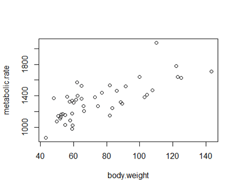
With the rmr data set, plot metabolic rate versus body weight. Fit a linear regression to the relation. According to the fitted model, what is the predicted metabolic rate for a body weight of 70 kg?
The data set rmr is R, make sure to install the book R package: ISwR. After installing the ISwR package, here is a simple illustration to the set of the problem. library(ISwR)plot(metabolic.rate~body.weight,data=rmr)
# 4) From our textbook Introductory Statistics pp. 124 Exercises # 6.1
#library(ISwR)
## Warning: package ‘ISwR’ was built under R version 4.2.3
plot(metabolic.rate~body.weight,data=rmr)
m_model <- lm(metabolic.rate ~ body.weight, data=rmr)
summary(m_model)
##
## Call:
## lm(formula = metabolic.rate ~ body.weight, data = rmr)
##
## Residuals:
## Min 1Q Median 3Q Max
## -245.74 -113.99 -32.05 104.96 484.81
##
## Coefficients:
## Estimate Std. Error t value Pr(>|t|)
## (Intercept) 811.2267 76.9755 10.539 2.29e-13 ***
## body.weight 7.0595 0.9776 7.221 7.03e-09 ***
## —
## Signif. codes: 0 ‘***’ 0.001 ‘**’ 0.01 ‘*’ 0.05 ‘.’ 0.1 ‘ ‘ 1
##
## Residual standard error: 157.9 on 42 degrees of freedom
## Multiple R-squared: 0.5539, Adjusted R-squared: 0.5433
## F-statistic: 52.15 on 1 and 42 DF, p-value: 7.025e-09
coeff <- coefficients(m_model)
coeff
## (Intercept) body.weight
## 811.226674 7.059528
bdweight <- 70
predictive_metabolic <- coeff[1] + coeff[2]* bdweight
predictive_metabolic # 70kg
## (Intercept)
## 1305.394
