I enjoyed this session a lot because it allows me to follow trends on current data.

A time series is like a sequence of data points that are collected or measured at regular intervals over time.

The Exponential Smoothing Model is a way to make predictions based on past values in a time series. It’s like trying to guess what the future data point will be based on the recent history.

# The data below represents charges for a student credit card.
# a. Construct a time series plot using R.

cc_charges <- c(31.9,27,31.3,31,39.4,40.7,42.3,49.5,45,50,50.9,58.5,39.4,36.2,40.5,44.6,46.8,44.7,52.2,54,48.8 ,55.8,58.7,63.4)
cc_timeseries <-ts(cc_charges)
cc_timeseries <-ts(cc_charges,frequency=12,start=c(2012,1))
cc_timeseries

##       Jan  Feb  Mar  Apr  May  Jun  Jul  Aug  Sep  Oct  Nov  Dec
## 2012 31.9 27.0 31.3 31.0 39.4 40.7 42.3 49.5 45.0 50.0 50.9 58.5
## 2013 39.4 36.2 40.5 44.6 46.8 44.7 52.2 54.0 48.8 55.8 58.7 63.4

#b. Employ Exponential Smoothing Model as outline in Avril VoghlanLinks to an external site.’s notes and report the statistical  outcome

cc_forecast<-HoltWinters(cc_timeseries)
cc_forecast

## Holt-Winters exponential smoothing with trend and additive seasonal component.
##
## Call:
## HoltWinters(x = cc_timeseries)
##
## Smoothing parameters:
##  alpha: 0.4786973
##  beta : 0
##  gamma: 0.1
##
## Coefficients:
##            [,1]
## a    51.4481469
## b     0.6088578
## s1   -6.6831338
## s2  -10.5867440
## s3   -6.6998393
## s4   -3.0320795
## s5   -1.4068647
## s6   -4.0422184
## s7    0.4727766
## s8    6.6378768
## s9    1.4431586
## s10   5.6809745
## s11   5.7999737
## s12  12.6976853

#c. Provide a discussion on time series and Exponential Smoothing Model result you led to.

# cc_forecast$fitted
#
# cc_forecast$SSE

plot(cc_forecast)

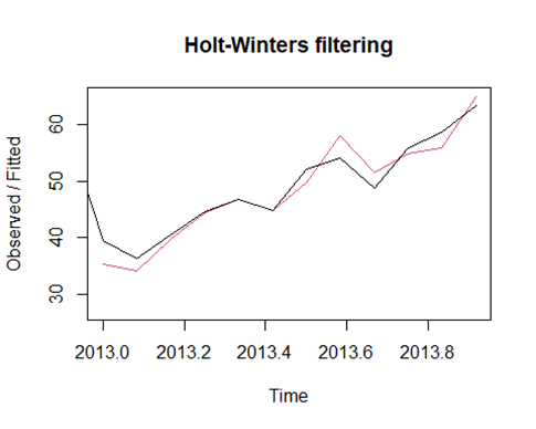
1. Model Type:

The modeling technique used is Holt-Winters exponential smoothing with the trend and additive seasonal component. It indicates that this model incorporates a trend (how the data changes over time) and an additive seasonal component (how the data follows a repeating pattern at certain intervals).

2. Smoothing Parameters:

 Alpha: 0.4786973 is the smoothing parameter for the level component of the model. It controls how much the model relies on recent data to estimate the current level.

Beta: 0 is the smoothing parameter for the trend component. The trend component doesn’t have a significant effect in this model.

Gamma: 0.1 is the smoothing parameter for the seasonal component. It determines how much the model relies on seasonal patterns to make predictions.

3. Coefficients:

These coefficients represent the estimated values for various components of the model.

   – “a” is the estimated time series level (the baseline).

   – “b” is the estimated slope or trend of the time series (how it’s changing over time).

   – “s1” to “s12” are coefficients representing the estimated seasonal effects for each of the 12 months (e.g., January to December). These values capture how the data tends to vary seasonally at each time of the year.

In simpler terms, this Holt-Winters model uses historical data to estimate the current level, trend, and seasonal patterns in the time series. It uses smoothing parameters (alpha, beta, and gamma) to determine how much recent data, trends, and seasonality should influence its predictions. The coefficients represent the estimated values for these components. This model can be used to make future predictions or understand the underlying patterns in the data.