Hello! This post explores matrix operations in R, specifically focusing on:

• Matrix arithmetic (addition and subtraction)
• Creating diagonal matrices using the diag() function
• Constructing custom matrices using diag() and sweep()

Let’s dive into hands-on R coding and learn how these fundamental concepts power data transformations!
NOTE: 📂 Check out my full code on GitHub!

---

1. Matrix Addition and Subtraction

We start by defining two matrices:

# Define matrices A and B

A <- matrix(c(2, 0, 1, 3), ncol = 2)

B <- matrix(c(5, 2, 4, -1), ncol = 2)

# Display matrices A and B

Matrices:

Matrix A:

     [,1] [,2]

[1,]    2    1

[2,]    0    3

Matrix B:

     [,1] [,2]

[1,]    5    4

[2,]    2   -1

---

 a) Matrix Addition (A + B)

# Matrix addition

A + B

Output:

     [,1] [,2]

[1,]    7    5

[2,]    2    2

---

 b) Matrix Subtraction (A – B)

# Matrix subtraction

A – B

Output:

     [,1] [,2]

[1,]   -3   -3

[2,]   -2    4

---

Explanation:

• Matrix addition and subtraction are performed element-wise in R.
• In simpler terms, R operates (like addition or subtraction) on each pair of elements located at the same position in the matrices.
• Each corresponding element in the matrices is added or subtracted directly.
• These operations require that matrices have compatible dimensions.

---

2. Creating a Diagonal Matrix with diag()

Let’s use diag() to create a 4×4 diagonal matrix with the values 4, 1, 2, 3 along its main diagonal.

💡R Code: Github

#Display diag_matrix

Output:

     [,1] [,2] [,3] [,4]

[1,]    4    0    0    0

[2,]    0    1    0    0

[3,]    0    0    2    0

[4,]    0    0    0    3

---

 Explanation:

• The diag() function takes a vector and places its values on the matrix’s main diagonal.
• The off-diagonal elements are automatically filled with zeros.
• Diagonal matrices are useful in many linear algebra applications, such as scaling and matrix transformations.

---

3. Constructing a Custom Matrix Using diag()

Target Matrix:

     [,1] [,2] [,3] [,4] [,5]

[1,]    3    1    1    1    1

[2,]    2    3    0    0    0

[3,]    2    0    3    0    0

[4,]    2    0    0    3    0

[5,]    2    0    0    0    3

---

💭 Challenge:

Initially, I attempted to solve this using a combination of diag() and sweep() for more dynamic row and column manipulations. However, after experimenting, I found that sweep() wasn’t efficiently providing the desired output. Instead, I opted for a straightforward approach using diag() combined with matrix indexing, which yielded the exact required matrix.

---

💡 Final R Code Solution: 📂 GitHub

---

Final Output:

     [,1] [,2] [,3] [,4] [,5]

[1,]    3    1    1    1    1

[2,]    2    3    0    0    0

[3,]    2    0    3    0    0

[4,]    2    0    0    3    0

[5,]    2    0    0    0    3

---

 Explanation:

• Step 1: The diag(3, 5, 5) function generates a 5×5 matrix with the value 3 along the main diagonal and 0 elsewhere.
• Step 2:
  • Row adjustment: I updated row 1, columns 2-5 to 1 using matrix indexing. This matches the pattern in the first row of the target matrix.
  • Column adjustment: I then updated column 1, rows 2-5 to 2, completing the required first column pattern.
• Step 3: I used diag() as a final confirmation to ensure that the diagonal values remained unchanged at 3.

---

💬 Reflection on the Approach:

While I initially considered using sweep() for a more dynamic solution, matrix indexing proved to be the most efficient and readable approach for this specific task. It allowed direct manipulation of the required elements, maintaining clarity and precision in the final output.

This exercise also reinforced the importance of flexibility in problem-solving—sometimes, the simplest solution is the most effective.

---

Conclusion:

The combination of diag() for creating the base matrix and matrix indexing for targeted adjustments provided a clean and intuitive solution. This method showcases how basic R functions can achieve complex transformations with minimal code when applied thoughtfully.

---

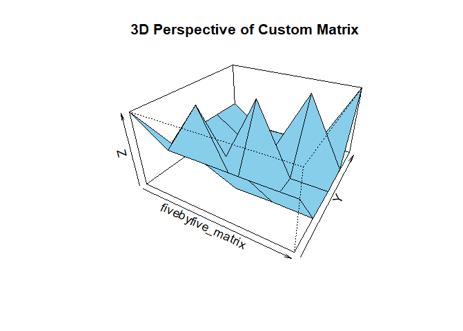
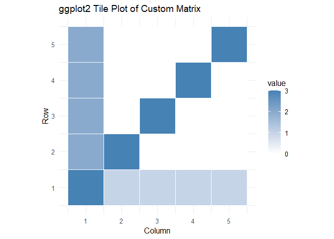
VISUALIZING!!!

Well, this blog is not final until I have shared some visualizations; I have asked AI if I can use the last assignment code (Constructing a Custom Matrix Using diag()), and of course, I can.

Please see my code at 📂 GitHub , here are some of the visualizations:

Final thoughts:

Visualizing matrices like this makes seeing patterns and interpreting relationships between elements easier. Plus, it adds a visual flair to my blog post!